Simulation Movies
Report Text
1. Introduction
On the morning of 26 August 2026 (local time), a large-scale debris flow and flood occurred near Langtang National Park along the Nepal-China border, apparently triggered by a rapid slope collapse involving glacier ice. The U.S. Geological Survey (USGS) provisionally summarized the event as the “2026 Nepal Debris Avalanche and Flash Flood” and reported that the flow traveled approximately 100 km along the Lende Khola-Trishuli Khola river system, causing major impacts on downstream settlements, roads, and bridges, including the Rasuwagadhi border facilities [1]. Reports published by The Kathmandu Post immediately after the disaster also stated that markets, settlements, and hydropower facilities around Timure and Syabrubesi were damaged, and warnings were issued for downstream areas along the Trishuli River [2].
This report presents an initial numerical reconstruction of this large-scale disaster using the Depth-Integrated Particle Method (DIPM) [3-8]. The simulated arrival times, travel distances, and particle-passage areas around major locations are compared with satellite imagery and interpreted damage areas. Based on these results, the effective material parameters of the moving mass are compared with those obtained for previous debris-flow events, and the distinctive characteristics of the present event are discussed. The report also considers possible approaches for risk assessment and damage mitigation for similar glacier-collapse-induced debris-flow events that may occur in the future.
2. Data Used in the Analysis
Topographic elevation data for the analysis were obtained from the Copernicus DEM GLO-30 GeoTIFF dataset [9]. The region between longitudes 84.949861111-85.649861111 and latitudes 27.800138889-28.500138889 was extracted from the original dataset. The original pixel dimensions are approximately 27.3 m x 30.8 m. The computational terrain was represented by a 2521 x 2521 grid with a grid spacing of 29.0 m. The elevation within the domain ranges from 382.5 to 7352.6 m.
For visualization of the analysis results, Esri World Imagery XYZ tiles were used for the regional-scale satellite imagery [10]. For identification of the collapse area and detailed comparisons between simulated inundation areas and the observed affected areas around individual towns, true-color images from Sentinel-2 Level-2A and Landsat Collection 2 Level-2 were used [11, 12].
Figure 1(a) shows the contour map generated from the elevation data, while Fig. 1(b) shows the satellite image of the same region together with the prescribed collapse area. Figure 2 shows the relationship between distance and elevation along the valley path indicated in Fig. 1.
Figure 3 shows the three-dimensional elevation data of the collapse area mapped with satellite imagery, together with the collapse area identified from the imagery and used in the analysis. The area is approximately 2.0 x 10^6 m2. Assuming mean collapse depths of 30 m, 50 m, and 100 m, the corresponding collapse volumes, including glacier ice, are 60.0 x 10^6 m3, 100.0 x 10^6 m3, and 200.0 x 10^6 m3, respectively. At present, however, published estimates of the collapse volume span a wide range. Park (2026) [13] used an initial collapse volume of 35.4 x 10^6 m3 in a flow analysis constrained by seismic timing, CCTV imagery, and river-monitoring records. In contrast, an inversion of long-period seismic waves by CLaSH/EarthScope [14] estimated a substantially larger collapse volume of approximately 197-492 x 10^6 m3. Thus, the collapse volume remains poorly constrained at present.
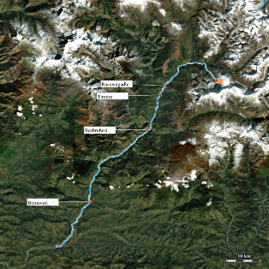
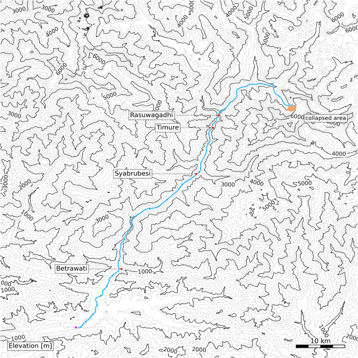
Fig. 1 Study area (Trishuli River basin along which the debris flow propagated)
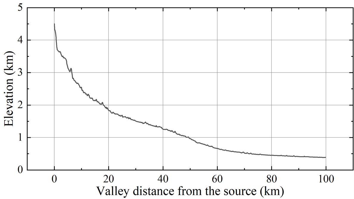
Fig. 2 Elevation profile along the valley path
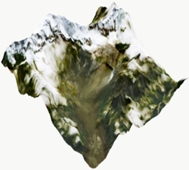
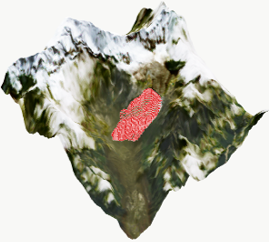
Fig. 3 Three-dimensional elevation model of the collapse area mapped with satellite imagery (left) and the collapse area identified from the imagery and prescribed in the analysis (right)
3. Outline of DIPM Analysis and Parameters Used
The Depth-Integrated Particle Method (DIPM) used in this study discretizes, by a particle method, the governing equations obtained by depth-integrating the flow field (also referred to as the shallow-water equations). Each computational particle is treated as a soil column of constant volume and moves under the effects of the topographic gradient, gravity, basal resistance, and interparticle interactions derived from the hydraulic-pressure gradient. A particular feature of the method is that interactions among computational particles are represented by the superposition of pairwise interactions with neighboring particles, allowing stable calculations with a relatively small number of particles. Consequently, even a large-scale flow extending approximately 100 km, such as the present event, can be analyzed on a personal computer in approximately 30 min per run, depending on the number of particles, making it possible to conduct many simulations with different calculation conditions over a short period. In addition, the present analysis restricts the principal flow-property parameters to only two quantities: Manning's roughness coefficient n, which is determined mainly by the conditions of the flow bed, and the critical deposition angle i_cr, the slope angle below which the flow stops (0 deg for water, and a value dependent on sediment properties and water content for a soil-water mixture). This makes it possible to perform analyses without detailed material properties of the sediment. Conversely, DIPM is not intended to pursue highly detailed local accuracy; rather, as discussed later, it is intended as a practical method for statistical evaluation of hazard over sediment-disaster-prone areas.
Previous studies have applied DIPM to post-Wenchuan-earthquake debris flows, the Atami debris flow, and wide-area slope-failure-induced debris flows in Atsuma Town following the Hokkaido Eastern Iburi Earthquake. Its reproducibility has been examined through comparison with real-terrain DEMs, satellite imagery, and field observations [3-8].
In this first report, the analysis cases listed in Table 1 were examined. A 29 m mesh was used over a 2521 x 2521 grid domain (approximately 73.1 km x 73.1 km). Initial collapse particles were arranged in a staggered pattern. A total of 1157 particles were used, and the initial height of each soil column was set to 60 m, corresponding to a total moving volume of 58.4 million m3. This initial column height was calculated from the prescribed number of columns and the total moving volume. Accordingly, reducing the initial column height also proportionally reduces the total moving volume and affects the subsequent decrease in column height during propagation. Once motion begins, the columns spread horizontally through interactions with surrounding particles, and their height decreases to approximately 10 m.
| Case No. | Manning coefficient, n | Critical deposition angle, i_cr (deg) | Initial mass height (m) |
|---|---|---|---|
| 01 | 0.02 | 0 | 60 |
| 02 | 0.03 | 0 | 60 |
| 03 | 0.04 | 0 | 60 |
| 04 | 0.03 | 0 | 30 |
| 05 | 0.03 | 0 | 15 |
| 06 | 0.03 | 0.5 | 60 |
| 07 | 0.03 | 1 | 60 |
4. Analysis Results
4.1 Arrival Time and Flow Velocity of the Debris Flow
Figure 4 shows the time history of the mean position of the ten leading particles for the analysis cases listed in Table 1. This quantity represents the travel distance of the debris-flow front along the valley path. The results show that when the critical deposition angle is greater than 0 deg, the flow stops before reaching the downstream end, whereas for a critical deposition angle of 0 deg, the flow continues to move in a manner similar to ordinary water flow. The results also show that the debris-flow velocity decreases as Manning's coefficient increases.
Arrival times at major locations have been reported in several investigations and news reports [15-17]. These data are summarized in Table 3 and compared with the numerical results in Fig. 4. The travel times are measured from the glacier-slope collapse time inferred by the USGS from seismic records [18]. Comparison with these observational estimates indicates that DIPM Case 1 or Case 2 (n = 0.02-0.03, i_cr = 0 deg) gives results that are relatively consistent with the observations. However, the reported arrival times contain uncertainties among different reports and observational records and should be reassessed as additional information becomes available.
The value i_cr = 0 deg indicates that the moving mass behaved with extremely high mobility and, in DIPM, is represented as having almost no effective yield resistance. As discussed later, this may reflect effects such as high water content, incorporation of glacier ice and meltwater, and mixing with river water.
As noted above, an initial mass height of 60 m corresponds to a collapse volume of 58.4 million m3. When this value is reduced by one-half or one-quarter (30 m or 15 m), the velocity of the debris-flow front decreases.
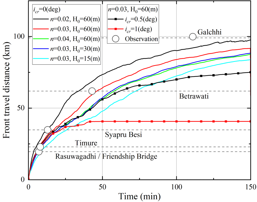
Fig. 4 Time history of debris-flow travel distance along the valley path
*1 Another estimation is 16 min according to Reference [14].
Figure 5 shows the relationship between the position of the debris-flow front and the flow velocity. For the cases that best match the available arrival-time observations (n = 0.02-0.03, i_cr = 0 deg), the initial front velocity reaches approximately 100 m/s and subsequently decreases to approximately 30 m/s at Rasuwagadhi and 25 m/s at Timure.
The local velocity peaks appear at similar locations for the different cases, suggesting that they are primarily controlled by changes in the topographic gradient.
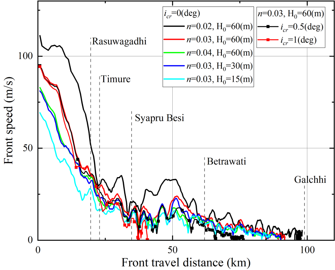
Fig. 5 Relationship between debris-flow front position and flow velocity
4.2 Flow Sequence for a Representative Case
Figure 6 shows the flow sequence for Case 2 (n = 0.03, i_cr = 0 deg). The moving mass follows the complex valley system downstream. In the present analysis, the water already flowing in the Trishuli River at the time of the event and the increase in sediment volume caused by riverbed erosion during the debris-flow passage are not taken into account.
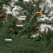
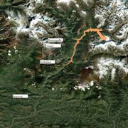
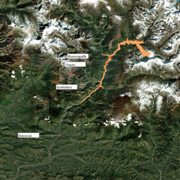
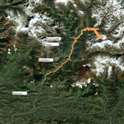
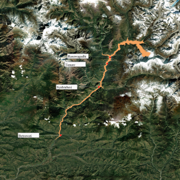
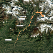
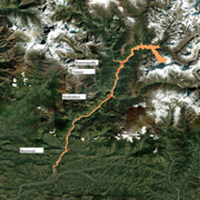
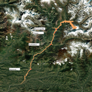
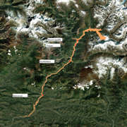
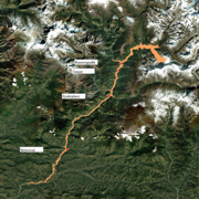
Fig. 6 Flow sequence for Case 2 (n = 0.03, i_cr = 0 deg, initial mass height = 60 m)
4.3 Comparison of Simulated Inundation Areas with Observed Affected Areas
Figure 7 compares satellite imagery of debris-flow deposits at several locations with the flow area obtained from DIPM Case 2. Overall, the simulated flow width is somewhat larger than the actual sediment-affected area. Possible reasons include the relatively coarse DEM pixel size (29 m) and the coarse representation of the initial collapse mass (1157 soil columns, each represented by an initial 29 m x 29 m x 60 m volume). The influence of using spatially uniform material parameters and the lateral particle-interaction model should also be examined in future work.
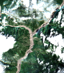
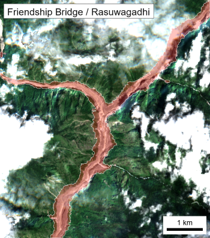
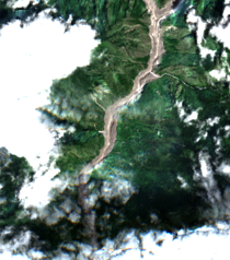
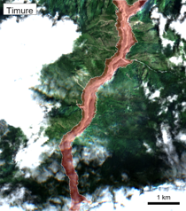
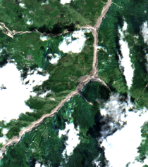
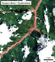
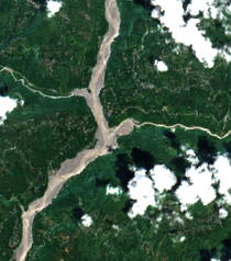
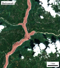
Fig. 7 Comparison of observed inundation/affected areas and DIPM results at selected locations
5. Comparison of Parameters with Previous Studies
In DIPM, Manning's coefficient n primarily controls the velocity-dependent component of basal resistance, whereas the critical deposition angle i_cr primarily controls the effective threshold for transition from motion to deposition or stoppage. Accordingly, n should be interpreted not only as a measure of channel-bed roughness but also as an effective parameter representing velocity-dependent resistance between the moving mass and the bed. Similarly, i_cr should be interpreted as an effective deposition/yield parameter that incorporates the effects of water content and flow mobilization.
Comparison of representative values identified in previous DIPM analyses with those obtained in the present study (Table 4) shows that both n and i_cr are very small for the Nepal event. In particular, i_cr is known to be strongly influenced by water content. The unusually long runout of more than 100 km and the extensive damage may have been influenced by the fact that the collapsed material included glacier ice and glacial deposits in addition to sediment, together with the high monsoon-season discharge of the Trishuli River.
6. Conclusions: Limitations of the Present Analysis and Future Work
This report presented an initial numerical reconstruction of the debris flow and flood triggered by a large-scale slope collapse involving glacier ice near the Nepal-China border on 26 August 2026. A regional-scale terrain model was constructed using Copernicus DEM data, and the event was analyzed using the Depth-Integrated Particle Method (DIPM). The approximately 100 km-long propagation was simulated within a single computational domain, and the results were compared with estimated arrival times at major locations, debris-flow/flood front velocities, and affected areas interpreted from satellite imagery.
Comparison with the currently available observational and reported information indicates that long-distance, high-speed propagation is reproduced relatively well for cases with a small Manning coefficient (n = 0.02-0.03) and a critical deposition angle close to 0 deg. Compared with representative values obtained in previous DIPM studies, the effective flow resistance and yield resistance required to reproduce this event are both relatively small. This suggests that the present event may have involved an exceptionally mobile moving mass, different from ordinary sediment-dominated debris flows, in which collapse material containing glacier ice and meltwater mixed with a large volume of river water during downstream propagation. However, as the arrival-time data are reassessed, the range of parameters that provides the best agreement may also need to be reconsidered.
The present analysis is a rapid first-stage assessment and several important uncertainties remain. First, estimated arrival times at major locations differ among CCTV records, river-gauge data, eyewitness accounts, and news reports, particularly in the upstream region, and therefore require further examination. Second, the initial collapse mass was simplified as a group of soil columns with uniform height; the actual spatial distribution of collapse thickness, the relative proportions of ice and sediment, and phase changes during motion were not considered. Third, the existing water flow in the Trishuli River, increases in moving volume due to riverbed erosion, inflow from tributaries, and downstream changes in material composition were not explicitly represented in the present model. These simplifications may influence the simulated propagation speed, runout extent, and inundation pattern, particularly as the flow moves downstream. Finally, local topographic and surface features such as buildings, structures, and vegetation are not explicitly represented at the 29 m DEM resolution which together with particle discretization, may affect the representation of flow paths and inundation widths and therefore require further investigation.
The present analysis demonstrates that, even using only globally available DEMs, satellite imagery, and limited observational information obtainable shortly after a disaster, DIPM can rapidly simulate the propagation of a debris-flow/flood event on the scale of 100 km. By progressively updating the analysis conditions as new observations become available, the method is intended to be developed as a rapid wide-area risk-assessment tool for similar glacier-collapse-induced debris flows and floods in high-mountain regions, with the ultimate aim of contributing to the mitigation of future disasters of this kind.
The authors extend their deepest sympathies to all those affected by this disaster and sincerely hope for the earliest possible recovery of the affected communities.
References
- U.S. Geological Survey, “2026 Nepal Debris Avalanche and Flash Flood”, Landslide Hazards Program, 2026. https://www.usgs.gov/programs/landslide-hazards/science/2026-nepal-debris-avalanche-and-flash-flood Back to text
- The Kathmandu Post, “Flash flood hits Rasuwa, damages hydropower projects and markets”, 26 August 2026. https://kathmandupost.com/national/2026/08/26/major-flood-damages-syabrubesi-hydropower-projects-in-rasuwa Back to text
- Zhang, N. and Matsushima, T.: “Simulation of rainfall-induced debris flow considering material entrainment,” Engineering Geology, Vol. 214, pp. 107–115, 2016. DOI: 10.1016/j.enggeo.2016.10.005. Back to text
- Zhang, N. and Matsushima, T.: “Numerical investigation of debris materials prior to debris flow hazards using satellite images,” Geomorphology, Vol. 308, pp. 54–63, 2018. DOI: 10.1016/j.geomorph.2018.02.008. Back to text
- Zhang, N., Matsushima, T. and Peng, N.: “Numerical investigation of post-seismic debris flows in the epicentral area of the Wenchuan earthquake,” Bulletin of Engineering Geology and the Environment, Vol. 78, No. 5, pp. 3253–3268, 2019. DOI: 10.1007/s10064-018-1359-6. Back to text
- Ahmed, M. E. and Matsushima, T.: “Evaluation of soil properties of natural slopes from case histories and GIS,” Proceedings of the International Conference on Computational Science (ICCS 2019), 12p, Singapore, 2019. Back to text
- Chowdhury, F. H. and Matsushima, T.: “Modeling the Atami debris flow using the depth-integrated particle method and GIS: Flow characteristics and future risk assessment,” Natural Hazards Research, Vol. 5, pp. 705–718, 2025. DOI: 10.1016/j.nhres.2025.03.008. Back to text
- Chowdhury, F. H. and Matsushima, T.: “Quantitative evaluation and wide-area simulation of post-failure debris flows using the depth-integrated particle method,” Geoenvironmental Disasters, Vol. 13, Article 17, 19p, 2026. DOI: 10.1186/s40677-025-00357-1. Back to text
- Copernicus Data Space Ecosystem, “Copernicus DEM - Global and European Digital Elevation Model”. https://dataspace.copernicus.eu/explore-data/data-collections/copernicus-contributing-missions/collections-description/COP-DEM Back to text
- Esri, “World Imagery MapServer”. https://services.arcgisonline.com/ArcGIS/rest/services/World_Imagery/MapServer Back to text
- European Space Agency (ESA) / European Commission, “Sentinel-2 Level-2A,” Copernicus Data Space Ecosystem, 2026. https://dataspace.copernicus.eu/data-collections/copernicus-sentinel-missions/sentinel-2 Back to text
- Earth Resources Observation and Science (EROS) Center, “Landsat 8–9 Operational Land Imager / Thermal Infrared Sensor Level-2, Collection 2,” U.S. Geological Survey, 2020. DOI: 10.5066/P9OGBGM6. https://www.usgs.gov/landsat-missions/landsat-collection-2-level-2-science-products Back to text
- Park, H.: “A rock-ice avalanche and the 2026 Bhote Koshi-Trishuli flood, Nepal,” EarthArXiv, preprint, 2026. DOI: 10.31223/X5250R. Back to text
- Center for Land Surface Hazards (CLaSH): “August 2026 Nepal Trishuli Flood,” StoryMap, updated 2 September 2026. Seismic volume estimates by Christopher Calvelage, EarthScope. https://storymaps.arcgis.com/stories/f2b2425eac544929a7d18f4c90b41d66 Back to text
- HiRISK, “A cascading high-mountain disaster: Rasuwa Flood, 26 August 2026,” Rapid Hazard Assessment, 2026. ( https://rasuwaflood.org/event.html) Back to text
- OnlineKhabar, “‘Nothing is left of Timure Bazaar’,” 26 Aug. 2026. ( https://english.onlinekhabar.com/nothing-is-left-of-timure-bazaar.html) Back to text
- Ram Kumar DC, “How the Bhotekoshi flood unfolded over 10 hours,” The Kathmandu Post, 27 August 2026; based on the initial technical report of the Flood Forecasting Division, Centre of Hydrology and Water Resources Research. (https://kathmandupost.com/national/2026/08/27/how-the-bhotekoshi-flood-unfolded-over-10-hours) Back to text
- U.S. Geological Survey (USGS), “M 5.2 Landslide – 55 km NW of Kodārī, Nepal,” USGS Earthquake Hazards Program, Earthquake Event Page, Event ID: us7000tbwb, 26 August 2026. Back to text